6. Convolution Neural Networks(CNN)
6.1. CNN Theory
- CNN이란?
- ANN은 Fully Connected Layer만으로 구성되어 있기 때문에, 입력 데이터는 1차원(배열) 형태로 입력되어야 한다(지난 ANN Implementation에서 reshape을 하는 이유 참조).
- 이미지나 영상 데이터는 흑백이 아닌 컬러 사진의 경우 3채널이기 때문에 3차원 데이터로 구성된다. 이를 ANN을 사용하려면 1차원으로 평면화시키는 과정에서 당연히 공간 정보가 손실될 수밖에 없다.
- 이러한 문제를 해결하는(이미지 공간 정보를 유지) 모델이 바로 CNN(Convolution Neural Network)이다.
- 특징
- 객체, 얼굴, 장면을 인식하기 위한 패턴을 찾는 데 유용하다.
- 2차원 이상의 데이터의 정보를 그대로 유지
- 복수의 필터를 사용하여 정보의 feature를 직접 학습하기 때문에 수동으로 feature를 추출할 필요가 없음.
- (convolution + pooling) 형태로 구성
- 필터를 공유 파라미터로 사용하기 때문에, 학습 파라미터가 적다.
- CNN은 결과값이 원하는 방향으로 설정(특징 a만 모으기, 특징 b만 모으기, …)할 수 있기 때문에 성능이 정말 좋다.
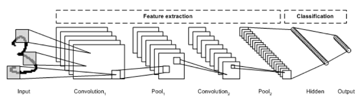
- 이미지의 feature를 추출하는 부분과 class를 분류하는 부분으로 나뉜다.
- feature 추출 영역: convolution layer, pooling layer
- class 분류 영역: fully connected layer
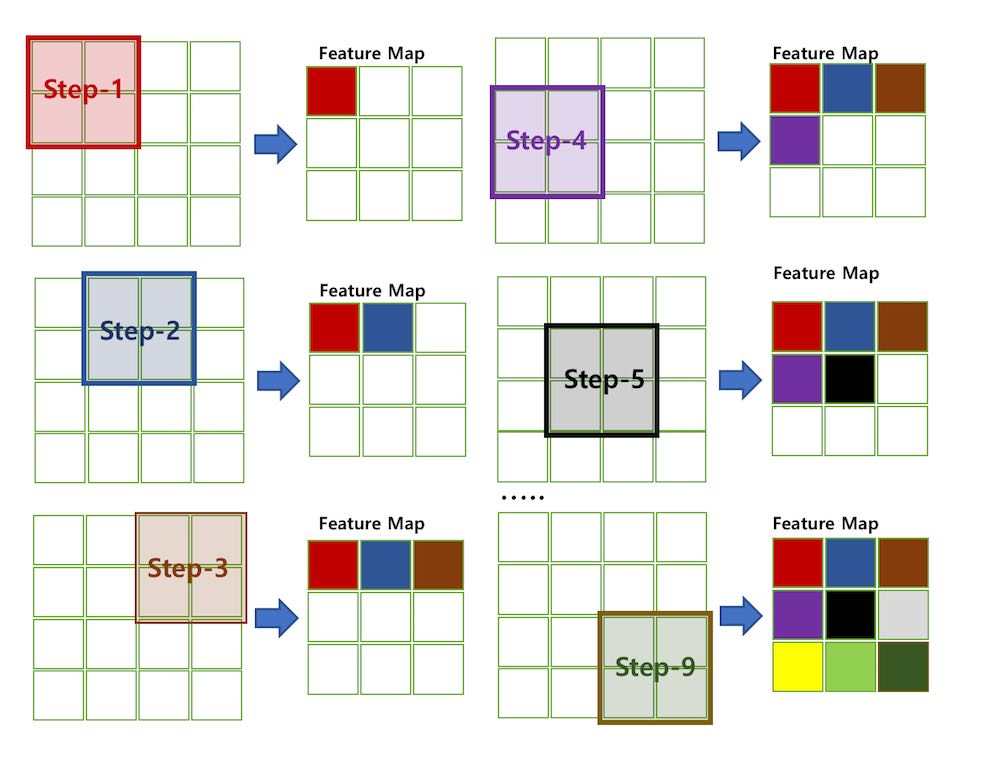
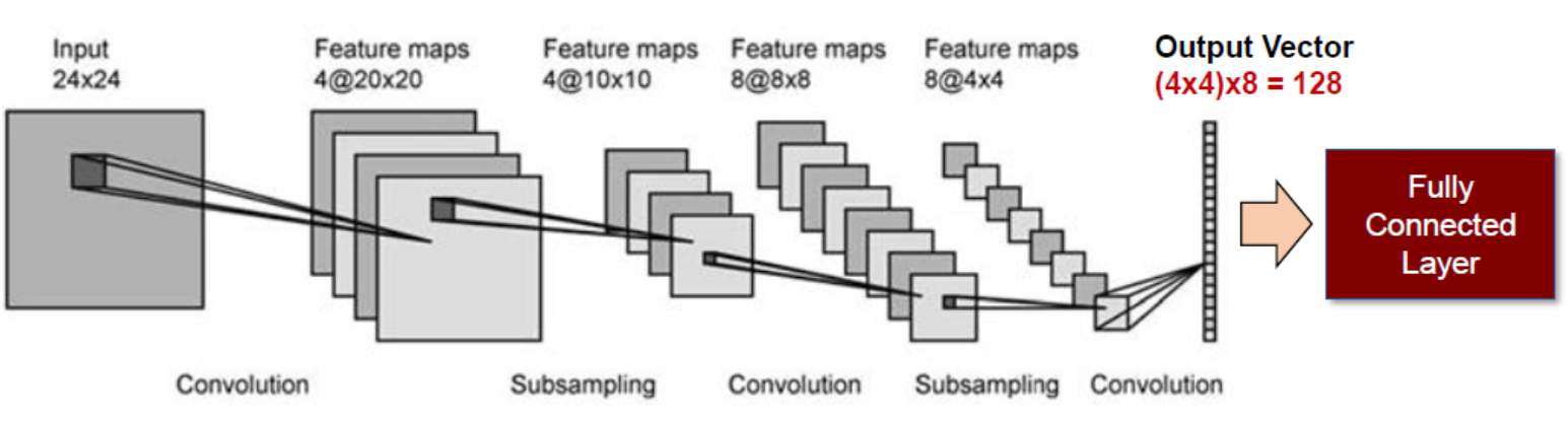
- 이미지의 feature를 추출하기 위해 입력 데이터를 필터(filter)가 순회하며 합성곱(convolution)을 계산하고, 그 계산 결과를 이용해 feature map을 만든다.
- convolution layer는 filter, stride, padding, pooling에 따라 출력 데이터의 shape이 달라진다.
-
CNN 주요 용어
1) 합성곱(Convolution)
- 합성곱 처리는 아래의 사진과 같으며, 그 결과로 Feature Map을 만든다.
- convolution layer에는 항상 Relu 함수가 함께 계산된다.
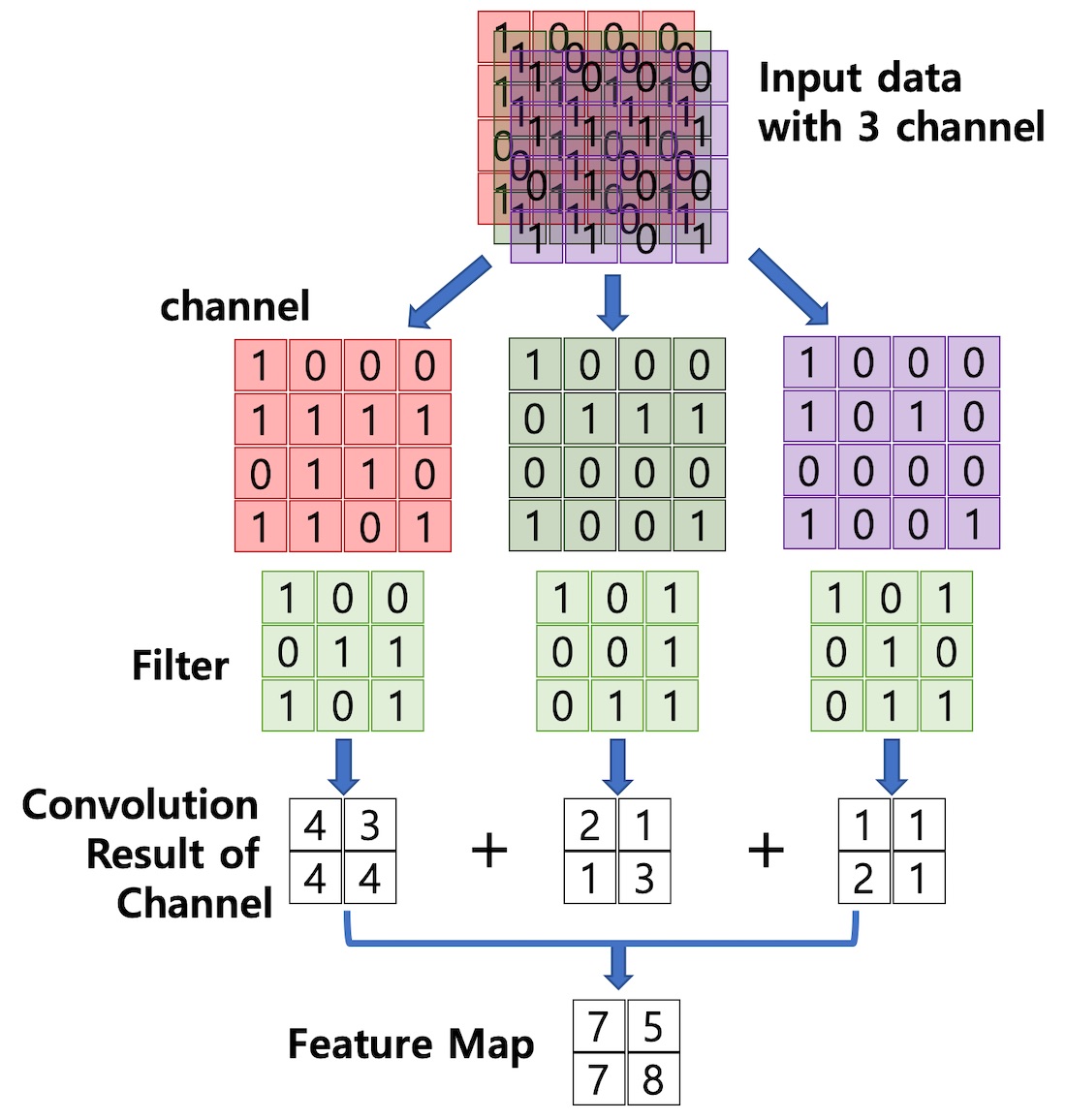
2) 채널(Channel)
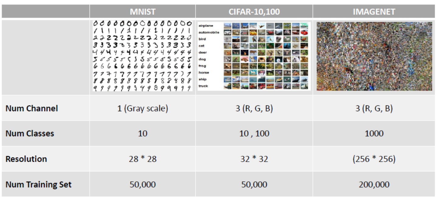
- 이미지의 픽셀의 값은 모두 실수이다. 각 픽셀은 RGB 3개의 실수로 표현한 3차원 데이터이다.
- 컬러 이미지는 3개의 채널로 구성도지만, 흑백 이미지는 1개의 채널로 구성된다.
- 합성곱 레이어에 유입되는 입력 데이터에는 한 개 이상의 필터가 적용된다. 만약, n개의 필터가 적용된다면 출력 데이터는 n개의 채널을 갖는다.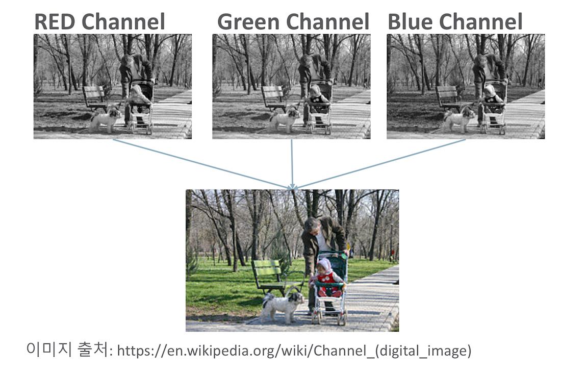
3) 필터(Filter) & 스트라이드(Stride)
- 필터는 이미지의 특징을 찾아내기 위한 공용 파라미터이다.
- CNN에서는 filter를 kernel과 같은 의미이다(OpenCV에서는 mask)
- 필터는 일반적으로 정사각 행렬로 정의되며, 입력 데이터를 지정된 간격으로 순회하며 채널별로 합성곱을 하고 모든 채널의 합성곱의 합을 feature map으로 만든다.
- 지정된 간격으로 필터를 순회하는 간격을 Stride라고 한다. Stride를 사용하면 정보는 조금 잃더라도 빠르게 학습이 가능하기 때문에, 대용량 데이터의 경우 자주 사용된다.
- 입력 데이터가 여러 채널을 갖을 경우(컬러 이미지, 영상) 필터는 각각의 채널을 순회하며 합성곱을 계산하고, 채널별 feature map을 만든다.
- 그리고 각 채널의 feature map을 합산하여 최종 feature map을 반환한다.
- 계산된 결과로 만들어진 feature map은 activation map이라고도 하며, convolution layer의 최종 출력 결과물이다(다음 단계는 pooling).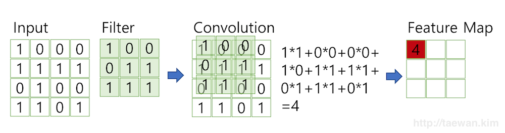
4) 패딩(Padding)
- OpenCV에서 mask 필터를 적용하면 이전의 이미지보다 압축된다는 것을 알 수 있다.
- 마찬가지로 convolution layer에서 filter와 stride를 적용하면서 feature map의 크기는 입력 데이터보다 작다.
- 이렇게 줄어드는 것을 방지하기 위해 사용하는 방법이 패딩(padding)이다.
- 패딩은 입력 데이터의 외각에 지정된 픽셀만큼 특정값으로 채워 넣는 것을 의미하며, 보통 0으로 채운다.
- 예를 들어 6x6 이미지의 1만큼의 패딩을 준다는 것은 6x6 이미지의 외곽을 1 픽셀만큼 더 크게 만드는 것으로, 이미지의 사이즈는 8x8이 된다.
이를 3x3 필터로 합성곱을 해주어도 그대로 6x6 이미지의 크기를 유지할 수 있다.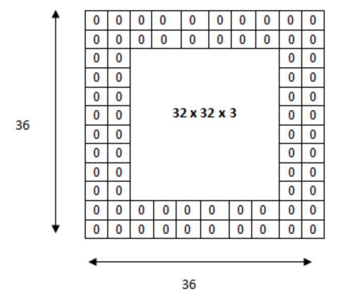
5) 풀링(Pooling)
- 풀링은 CNN의 구성 중 2단계에 해당하는 layer로, convolution layer의 출력 데이터(feature map, activation map)를 입력으로 받아서 크기를 줄이거나 특정 데이터를 강조하는 용도로 사용한다.
- 풀링의 방법은 Max Pooling, Average Pooling, Min Pooling이 있다.
- 정사각 행렬의 특정 영역 안에 값의 최댓값/평균값/최솟값을 구하는 방식으로 동작한다.
- pooling layer는 convolution layer에 비해 학습 파라미터가 없으며, 행렬의 크기가 감소한다는 특징이 있다.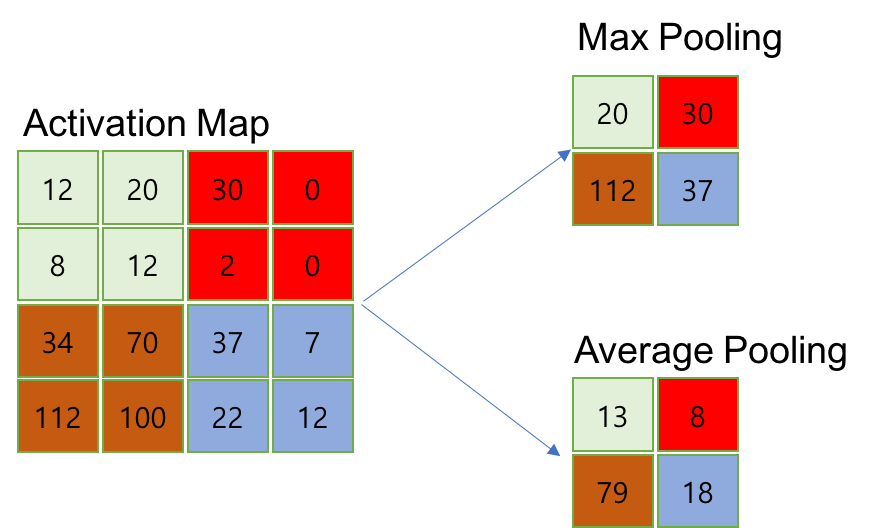
- CNN 구성
6.2. CNN Implementation
MNIST 데이터 분류하기
Tensorflow
from tensorflow.examples.tutorials.mnist import input_data
mnist = input_data.read_data_sets('MNIST_data/', one_hot=True)
import tensorflow as tf
import time
training_epochs = 15
batch_size = 100
X = tf.placeholder(tf.float32, [None, 784]) # MNIST의 이미지 사이즈는 28x28 = 784
Y = tf.placeholder(tf.float32, [None, 10]) # 라벨링은 0~9까지의 10개
X_img = tf.reshape(X, [-1, 28, 28, 1]) # 전체 사이즈(-1)를 받을 수 있도록, 28x28사이즈로, 1채널(흑백 이미지이므로, 컬러 이미지는 3채널로 변경)
# Convolution Layer 1
W1 = tf.Variable(tf.random_normal([3, 3, 1, 32], stddev=0.01)) # 하나의 이미지(1)를 3x3 사이즈의 32개 필터로 설정
CL1 = tf.nn.conv2d(X_img, W1, strides=[1, 1, 1, 1], padding='SAME') # stride에서 맨 앞과 맨 뒤는 의미가 없고, 1x1 간격으로 계산한다, padding에서 SAME은 패딩을 해준다 / VALID는 패딩을 안해준다의 뜻이다.
CL1 = tf.nn.relu(CL1) # convolution layer의 마지막에는 항상 relu 함수를 사용
# Pooling Layer 1
PL1 = tf.nn.max_pool(CL1, ksize=[1, 2, 2, 1], strides=[1, 2, 2, 1], padding='SAME') # 마찬가지로 ksize 역시 맨 앞과 맨 뒤는 의미가 없다. 2x2의 max pooling을 사용하여 반으로 나눈다는 뜻이다. ksize만큼 strides도 써준다.
# Convolution Layer 2
W2 = tf.Variable(tf.random_normal([3, 3, 32, 64], stddev=0.01)) # 32개의 이미지(32)를 3x3 사이즈의 64개 필터로 설정(0.01 표준편차는 0~9까지라는 것을 알기 때문)
CL2 = tf.nn.conv2d(PL1, W2, strides=[1, 1, 1, 1], padding='SAME')
CL2 = tf.nn.relu(CL2)
# Pooling Layer 2
PL2 = tf.nn.max_pool(CL2, ksize=[1, 2, 2, 1], strides=[1, 2, 2, 1], padding='SAME')
# Fully Connected Layer
L_flat = tf.reshape(PL2, [-1, 7*7*64]) # 처음 이미지의 사이즈는 28x28이었지만, Conv 1을 통과하면서 pooling 1에 의해서 반으로 줄어들고(14x14), 다시 Conv 2를 통과하면서 pooling 2에 의해서 반으로 줄어듦(7x7)
W3 = tf.Variable(tf.random_normal([7*7*64, 10], stddev=0.01))
b3 = tf.Variable(tf.random_normal([10]))
# # 더 간결하게
# # Convolution Layer1
# CL1 = tf.layers.conv2d(inputs=X_img, filters=32, kernel_size=[3, 3], padding='SAME', strides=1, activation=tf.nn.relu)
# # Pooling Layer1
# PL1 = tf.layers.max_pooling2d(inputs=CL1, pool_size=[2, 2], padding='SAME', strides=2)
# Convolution Layer2
# CL2 = tf.layers.conv2d(inputs=PL1, filters=64, kernel_size=[3, 3], padding='SAME', strides=1, activation=tf.nn.relu)
# # Pooling Layer2
# PL2 = tf.layers.max_pooling2d(inputs=CL2, pool_size=[2, 2], padding='SAME', strides=2)
# # Fully Connected (FC) Layer
# L_flat = tf.reshape(PL2, [-1, 7*7*64])
# W3 = tf.Variable(tf.random_normal([7*7*64, 10], stddev=0.01))
# b3 = tf.Variable(tf.random_normal([10]))
# Model, Cost, Train
model_LC = tf.add(tf.matmul(L_flat, W3), b3)
model = tf.nn.softmax(model_LC)
cost = tf.reduce_mean(tf.nn.softmax_cross_entropy_with_logits_v2(logits=model_LC, labels=Y))
train = tf.train.AdamOptimizer(0.01).minimize(cost)
# Accuracy
accuracy = tf.reduce_mean(tf.cast(tf.equal(tf.argmax(model, 1), tf.argmax(Y, 1)), tf.float32))
# Session
with tf.Session() as sess:
sess.run(tf.global_variables_initializer())
# Training
t1 = time.time()
for epoch in range(training_epochs):
total_batch = int(mnist.train.num_examples / batch_size)
for i in range(total_batch):
train_images, train_labels = mnist.train.next_batch(batch_size)
c, _ = sess.run([cost, train], feed_dict={X: train_images, Y: train_labels})
if i % 10 == 0:
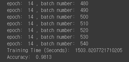
print('epoch: ', epoch, ', batch number: ', i)
t2 = time.time()
# Testing
print('Training Time (Seconds): ', t2 - t1)
print('Accuracy: ', sess.run(accuracy, feed_dict={X: mnist.test.images, Y: mnist.test.labels}))
Keras
from keras.utils import np_utils
from keras.datasets import mnist
from keras.models import Sequential
from keras.layers import Conv2D, pooling, Flatten, Dense
# MNIST data
(train_images, train_labels), (test_images, test_labels) = mnist.load_data()
print(train_images.shape, train_labels.shape, test_images.shape, test_labels.shape)
train_images = train_images.reshape(train_images.shape[0], 28, 28, 1).astype('float32')/255.0
test_images = test_images.reshape(test_images.shape[0], 28, 28, 1).astype('float32')/255.0
train_labels = np_utils.to_categorical(train_labels)
test_labels = np_utils.to_categorical(test_labels)
# Model
model = Sequential()
model.add(Conv2D(32, (3, 3), padding='same', strides=(1, 1), activation='relu', input_shape=(28, 28, 1)))
print(model.output_shape)
model.add(pooling.MaxPooling2D(pool_size=(2, 2)))
print(model.output_shape)
model.add(Conv2D(64, (3, 3), padding='same', strides=(1, 1), activation='relu'))
print(model.output_shape)
model.add(pooling.MaxPooling2D(pool_size=(2, 2)))
print(model.output_shape)
model.add(Flatten())
model.add(Dense(10, activation='softmax'))
model.compile(loss='categorical_crossentropy', optimizer='sgd', metrics=['accuracy'])
# Training
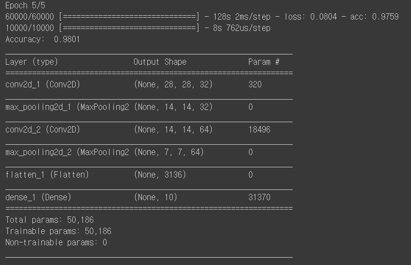
model.fit(train_images, train_labels, epochs=5, batch_size=100, verbose=1)
# Testing
_, accuracy = model.evaluate(test_images, test_labels)
print('Accuracy ', accuracy)
model.summary()
CIFAR-10 데이터 분류하기
Tensorflow
from keras.utils import np_utils
from keras.datasets import cifar10
import tensorflow as tf
import time

(train_images, train_labels), (test_images, test_labels) = cifar10.load_data()
train_labels = np_utils.to_categorical(train_labels)
test_labels = np_utils.to_categorical(test_labels)

training_epochs = 15
batch_size = 100

X = tf.placeholder(tf.float32, [None, 32, 32, 3])
Y = tf.placeholder(tf.float32, [None, 10])
X_img = tf.reshape(X, [-1, 32, 32, 3])

# Convolution Layer 1
W1 = tf.Variable(tf.random_normal([3, 3, 3, 32], stddev=0.01))
CL1 = tf.nn.conv2d(X_img, W1, strides=[1, 1, 1, 1], padding='SAME')
CL1 = tf.nn.relu(CL1)

# Pooling Layer 1
PL1 = tf.nn.max_pool(CL1, ksize=[1, 2, 2, 1], strides=[1, 2, 2, 1], padding='SAME')

# Convolution Layer 2
W2 = tf.Variable(tf.random_normal([3, 3, 32, 64], stddev=0.01))
CL2 = tf.nn.conv2d(PL1, W2, strides=[1, 1, 1, 1], padding='SAME')
CL2 = tf.nn.relu(CL2)

# Pooling Layer 2
PL2 = tf.nn.max_pool(CL2, ksize=[1, 2, 2, 1], strides=[1, 2, 2, 1], padding='SAME')

# Fully Connected Layer
L_flat = tf.reshape(PL2, [-1, 8*8*64])
W3 = tf.Variable(tf.random_normal([8*8*64, 10], stddev=0.01))
b3 = tf.Variable(tf.random_normal([10]))

# Model, Cost, Train
model_LC = tf.matmul(L_flat, W3) + b3
model = tf.nn.softmax(model_LC)
cost = tf.reduce_mean(tf.nn.softmax_cross_entropy_with_logits_v2(logits=model_LC, labels=Y))
train = tf.train.AdamOptimizer(0.01).minimize(cost)

# Accuracy
accuracy = tf.reduce_mean(tf.cast(tf.equal(tf.argmax(model, 1), tf.argmax(Y, 1)), tf.float32))

# Session
with tf.Session() as sess:
  sess.run(tf.global_variables_initializer())

  # Training
  t1 = time.time()
  for epoch in range(training_epochs):
    total_batch = int(train_images.shape[0] / batch_size)
    for i in range(total_batch):
      batch_train_images = train_images[i*batch_size : (i+1)*batch_size]
      batch_train_labels = train_labels[i*batch_size : (i+1)*batch_size]
      c, _ = sess.run([cost, train], feed_dict={X: batch_train_images, Y: batch_train_labels})

      if i % 10 == 0:
        print('epoch: ', epoch, ', batch number: ', i)

  t2 = time.time()

  # Testing
  print('Training Time (Seconds): ', t2 - t1)

  total_batch = int(test_images.shape[0] / batch_size)
  for i in range(total_batch):
    batch_test_images = test_images[i*batch_size : (i+1)*batch_size]
    batch_test_labels = test_labels[i*batch_size : (i+1)*batch_size]

  print('Accuracy: ', sess.run(accurcay, feed_dict={X: batch_test_images, Y: batch_test_labels}))
CIFAR-10 Dataset은 현재 노트북으로 실행 불가능
Keras
# 138p에 6번 7번 사이에 train_images test_images 255로 나눈 것 추가
from keras.utils import np_utils
from keras.datasets import cifar10
from keras.models import Sequential
from keras.layers import Conv2D, pooling, Flatten, Dense

(train_images, train_labels), (test_images, test_labels) = cifar10.load_data()
print(train_images.shape, train_labels.shape, test_images.shape, test_labels.shape)

# mnist 데이터와는 다르게 cifar10 데이터는 이미 shape에 3채널이 있기 때문에 reshpae을 할 필요는 없다
# 0과 1로 변환하여야 하기 때문에 255로 나눈다
train_images = train_images.reshape(train_images.shape[0], 32, 32, 3).astype('float32') / 255.0
test_images = test_images.reshape(test_images.shape[0], 32, 32, 3).astype('float32') / 255.0

train_labels = np_utils.to_categorical(train_labels)
test_labels = np_utils.to_categorical(test_labels)

model = Sequential()
model.add(conv2D(32, (3, 3), padding='same', strides=(1, 1), activation='relu', input_shape=(32, 32, 3)))
model.add(pooling.MaxPooling2D(pool_size=(2, 2)))
model.add(conv2D(64, (3, 3), padding='same', strides=(1, 1), activation='relu'))
model.add(pooling.MaxPooling2D(pool_size=(2, 2)))
model.add(Flatten())
model.add(Dense(10, activation='softmax'))
model.compile(loss='categorical_crossentropy', optimizer='sgd', metrics=['accuracy'])

model.fit(train_images, train_labels, epochs=5, batch_size=100, verbose=1)
_, accuracy = model.evaluate(test_images, test_labels)
print('Accuracy: ', accuracy)
model.summary()