딥 러닝을 이용한 자연어 처리 입문
Deep Learning for NLP 1 [TFIDF and NLP Objective]
1. TF-IDF
- 언어적인 특성을 반영하여 단어를 수치화하는 방법은 벡터를 사용하는 것이다.
- 데이터를 표현할 때 기본적으로 one-hot encoding 방식을 사용한다.
- 하지만 이 방식은 단어의 의미나 특성을 표현할 수 없으며, 단어의 수가 매우 많아지면 고차원 저밀도 벡터를 구성한다.
- 벡터의 크기가 작으면서 단어의 의미를 표현해줄 수 있는 방식이 필요하다.
- 분포가설에 기반하여, 같은 문맥의 단어(비슷한 위치에 나오는 단어)는 비슷한 의미를 가지는 특징을 사용하여 두 가지 표현법이 있다.
1) 카운트 기반 방법: 특정 문맥 안에서 단어들이 동시에 등장하는 횟수를 직접 센다.
2) 예측 방법: 신경망 등을 통해 문맥 안의 단어들을 예측한다.
- TF-IDF(Term Frequency-Inverse Document Frequency)는 단어의 빈도와 역문서 빈도(문서의 빈도에 특정 식을 취함)를 사용하여 DTM 내의 각 단어들마다 중요한 정도를 가중치로 주는 방법이다.
- DTM(Document-Term Matrix, 문서 단어 행렬)이란, 다수의 문서에서 등장하는 각 단어들의 빈도를 행렬로 표현하는 것이다.
- tf(d, t): 특정 문장(d)에서 특정 단어(t)가 몇 번 나오는지
- df(t): 특정 단어(t)가 등장한 문장의 수
- idf(d, t): df(t)에 반비례하는 수
- TF-IDF는 모든 문서에서 자주 등장하는 단어는 중요도가 낮다고 판단하며, 특정 문서에서만 자주 등장하는 단어는 중요도가 높다고 판단한다.
- TF-IDF 값이 낮으면 중요도가 낮은 것이고, 값이 크면 중요도가 큰 것이다. 즉, the나 a와 같은 불용어는 모든 문서에서 자주 나타나기 때문에 TF-IDF의 값이 다른 단어에 비해 낮다.
1.1. 사이킷런을 이용한 TF-IDF
from sklearn.feature_extraction.text import TfidfVectorizer
corpus = [
    'you know I want your love',
    'I like you',
    'what should I do ',
]
tfidfv = TfidfVectorizer().fit(corpus)
print(tfidfv.transform(corpus).toarray())
print(tfidfv.vocabulary_)
2. 문서 유사도
2.1. 자카드 유사도
- A와 B 두 개의 집합이 있을 때, 교집합은 두 개의 집합에서 공통으로 가지고 있는 원소들의 집합이다.
- 합집합에서 교집합의 비율을 구한다면, 두 집합 A와 B의 유사도를 구할 수 있다는 것이 자카드 유사도의 아이디어다.
- A / B
- A: 두 집합의 교집합인 공통된 단어의 개수(unique)
- B: 집합이 가지는 단어의 개수
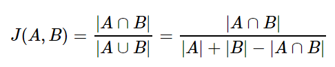
- 장점: 벡터를 사용하는 방법을 몰라도 사용 가능하다.
- 단점: 계란이나 달걀은 같은 단어이지만, 자카드 유사도는 0과 1로만 나타내기 때문에 유사도가 떨어진다.
#%%

doc1 = "apple banana everyone like likey watch card holder"
doc2 = "apple banana coupon passport love you"

tokenized_doc1 = doc1.split()
tokenized_doc2 = doc2.split()

print(tokenized_doc1)
print(tokenized_doc2)

#%%

# 문서1과 문서2의 합집합
union = set(tokenized_doc1).union(set(tokenized_doc2))
print(union)

#%%

# 문서1과 문서2의 교집합
intersection = set(tokenized_doc1).intersection(set(tokenized_doc2))
print(intersection)

#%%

print(len(intersection) / len(union))
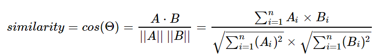
2.2. 코사인 유사도
- 코사인 유사도는 두 개의 벡터값에서 코사인 각도를 구하는 방법이다. 두 벡터의 방향이 동일한 경우 1의 값을 가지며, 90도의 각을 가지면 0, 180도로 반대의 방향을 가지면 -1의 값을 갖게 된다.
- 즉, -1과 1사이의 값을 가지며 1에 가까울수록 비슷하다.
#%%

import numpy as np
from sklearn.feature_extraction.text import TfidfVectorizer

sent = {"휴일인 오늘도 서쪽을 중심으로 폭염이 이어졌는데요, 내일은 반가운 비 소식이 있습니다.", "피해서 휴일에 놀러왔다가 갑작스런 비로 인해 망연자실하고 있습니다."}

tfidf_vectorizer = TfidfVectorizer()
tfidf_matrix = tfidf_vectorizer.fit_transform(sent)

print(tfidf_matrix)
print('First sentence')
print(tfidf_matrix[0])
print('Second sentence')
print(tfidf_matrix[1])

# Cosine similarity
from sklearn.metrics.pairwise import cosine_similarity
print('Cosine similarity: ', cosine_similarity(tfidf_matrix[0], tfidf_matrix[1]))

#%%

sent = {"영희가 눈물을 훔치며, 말을 이어나갔다.", "철수가 닭똥같은 눈물을 흐리며, 말을 멈추었다."}

tfidf_vectorizer = TfidfVectorizer()
tfidf_matrix = tfidf_vectorizer.fit_transform(sent)

print(tfidf_matrix)
print('First sentence')
print(tfidf_matrix[0])
print('Second sentence')
print(tfidf_matrix[1])
print('Cosine similarity: ', cosine_similarity(tfidf_matrix[0], tfidf_matrix[1]))

#%%

sent = {"밥을 먹는다", "밥을 먹다", "밥을 먹었다"}

tfidf_vectorizer = TfidfVectorizer()
tfidf_matrix = tfidf_vectorizer.fit_transform(sent)

print(tfidf_matrix)
print('First sentence')
print(tfidf_matrix[0])
print('Second sentence')
print(tfidf_matrix[1])
print('Third sentence')
print(tfidf_matrix[2])

print('Cosine similarity: ', cosine_similarity(tfidf_matrix[0], tfidf_matrix[1]))
print('Cosine similarity: ', cosine_similarity(tfidf_matrix[0], tfidf_matrix[2]))
print('Cosine similarity: ', cosine_similarity(tfidf_matrix[1], tfidf_matrix[2]))

#%%

from numpy import dot
from numpy.linalg import norm
import numpy as np

def cos_sim(A, B):
  return dot(A, B)/(norm(A)*norm(B))

# 밥을 / 먹는다 / 먹다 / 먹었다
doc1=np.array([1,0,0,0])
doc2=np.array([1,0,1,0])
doc3=np.array([1,0,0,1])

print(cos_sim(doc1, doc2))
print(cos_sim(doc1, doc3))
print(cos_sim(doc2, doc3))
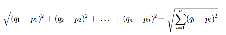
2.3. 유클리디언 유사도
- 유클리드 거리는 문서의 유사도를 구할 때 자카드 유사도나 코사인 유사도에 비해 유용한 방법은 아니다.
- 다차원 공간에서 두 점 사이의 거리를 계산하는 유클리드 거리 공식
#%%

import numpy as np
def dist(x, y):
  return np.sqrt(np.sum((x-y)**2))

doc1 = np.array((2, 3, 0, 1))
doc2 = np.array((1, 2, 3, 1))
doc3 = np.array((2, 1, 2, 2))
docQ = np.array((1, 1, 0, 1))

print(dist(doc1, docQ))
print(dist(doc2, docQ))
print(dist(doc3, docQ))
Deep Learning for NLP 2 [Text Understanding]
IMDB 영화 리뷰 데이터 처리
#%%

import os
import re
import pandas as pd
import tensorflow as tf
from tensorflow.keras import utils

# IMDB 데이터 다운로드
data_set = tf.keras.utils.get_file(
    fname="imdb.tar.gz",
    origin="http://ai.stanford.edu/~amaas/data/sentiment/aclImdb_v1.tar.gz",
    extract=True
)

def directory_data(directory):
  data = {}
  data["review"] = []
  for file_path in os.listdir(directory):
    with open(os.path.join(directory, file_path), "r", encoding="utf-8") as file:
      data["review"].append(file.read())
  return pd.DataFrame.from_dict(data)

def data(directory):
  pos_df = directory_data(os.path.join(directory, "pos"))
  neg_df = directory_data(os.path.join(directory, "neg"))
  pos_df["sentiment"] = 1
  neg_df["sentiment"] = 0
  return pd.concat([pos_df, neg_df])

train_df = data(os.path.join(os.path.dirname(data_set), "aclImdb", "train"))
test_df = data(os.path.join(os.path.dirname(data_set), "aclImdb", "test"))

#%%

train_df.head()

#%%

reviews = list(train_df["review"])

# 문자열 문장 리스트를 토큰화
tokenized_reviews = [r.split() for r in reviews]
# 토큰화된 리스트에 대한 각 길이를 저장(단어의 길이)
review_by_token = [t for t in tokenized_reviews]
review_len_by_token = [len(t) for t in tokenized_reviews]
# 토큰화된 것을 붙여서 음절의 길이를 저장(문장의 길이 - 공백을 제거해서 그냥 한줄로 표현)
review_by_alphabet = [s.replace(' ', '') for s in reviews]
review_len_by_alphabet = [len(s.replace(' ', '')) for s in reviews]

#%%

print(tokenized_reviews[:10])

#%%

print(review_by_token[:10])

#%%

print(review_len_by_token[:10])

#%%

print(review_by_alphabet[:10])

#%%

print(review_len_by_alphabet[:10])

#%%

import matplotlib.pyplot as plt
# 이미지 사이즈 선언, figsize: [가로, 세로] 형태의 튜플로 입력
plt.figure(figsize=(12, 5))

# 히스토그램 선언
# bins: 히스토그램 값들에 대한 버켓 범위
# range: x축 값의 범위
# alpha: 그래프 색상 투명도
# color: 그래프 색상
# label: 그래프에 대한 라벨
plt.hist(review_len_by_token, bins=50, alpha=0.5, color='r', label='word')
plt.hist(review_len_by_alphabet, bins=50, alpha=0.5, color='b', label='alphabet')

# 그래프 제목, x축 라벨, y축 라벨
plt.title("Review Length Histogram")
plt.xlabel("Review Length")
plt.ylabel("Number of Review")

#%% md

단어는 2,000개밖에 쓰지 않았지만, 문장의 길이는 훨씬 더 많다는 것을 알 수 있다.

#%%

import numpy as np

print("문장 최대길이: ", np.max(review_len_by_token))
print("문장 최소길이: ", np.min(review_len_by_token))
print("문장 평균길이: ", np.mean(review_len_by_token))
print("문장 길이 표준편차: ", np.std(review_len_by_token))
print("문장 중간길이: ", np.median(review_len_by_token))

# 사분위의 대한 경우는 0~100 스케일로 되어있음
print("제 1 사분위 길이: ", np.percentile(review_len_by_token, 25)) # 1/4의 위치(하위 25%)
print("제 3 사분위 길이: ", np.percentile(review_len_by_token, 75)) # 3/4의 위치(상위 25%)

#%% md

### 문장 내 단어 수에 대한 히스토그램

#%%

plt.figure(figsize=(12, 5))
# 박스플롯 생성
# 첫 번재 파라미터: 여러 분포에 대한 데이터 리스트를 입력
# labels: 입력한 데이터에 대한 라벨
# showmeans: 평균값을 마크함
plt.boxplot([review_len_by_token], labels=['token'], showmeans=True)

#%% md

### 문장 내 알파벳 수에 대한 히스토그램

#%%

plt.figure(figsize=(12, 5))
plt.boxplot([review_len_by_alphabet], labels=['alphabet'], showmeans=True)

#%%

from wordcloud import WordCloud, STOPWORDS

my_stopwords = STOPWORDS.add("br")
wordcloud = WordCloud(stopwords=STOPWORDS, background_color='black', width=800, height=600).generate(" ".join(train_df["review"]))

plt.figure(figsize=(15, 10))
plt.imshow(wordcloud)
plt.axis("off")
plt.show()

#%% md

### 긍정/부정의 분포 확인

#%%

import seaborn as sns

sentiment = train_df["sentiment"].value_counts()
fig, axe = plt.subplots(ncols=1)
fig.set_size_inches(6, 3)
sns.countplot(train_df["sentiment"])
plt.show()